Your Model Fits. Why Does Your Conversation Run Out of Memory?
Build a memory budget for a 128 GB Halo: weights, attention state, runtime buffers, and several people asking questions at once.
Our coding assistant has answered where invoice editing is authorized. You ask it to inspect the tests, then compare a background job, then explain a proposed change. The model loaded successfully at the beginning. Why does a later request run out of memory?
Because the model file was never the whole memory budget. The conversation grows, tools return more source code, and the server holds state while generating each answer. When a colleague starts another conversation, some allocations can be shared and others cannot.
Part one introduced weights, prefill, decode, and the attention cache. Here we put them into a capacity ledger. Every worked number is an illustrative calculation. A “128 GB Halo” is the hardware class being considered, not a machine whose available memory we have measured.
New to the terminology? Use the AI glossary. Linked terms also show a definition on hover or keyboard focus.
Start with an accounting identity
A useful first budget is:
Memory the inference process can actually use
  = resident weights
  + active request state, including KV cache
  + retained reusable cache blocks
  + runtime workspace and allocation overhead
  + unused safety headroom

Installed system memory
  also serves the OS, display, other processes and reservations.
Avoid double-counting: an active request can reference the same cache blocks that are retained for reuse. In a real allocator, measure unique resident allocations rather than adding overlapping dashboard totals.
Shared memory on a Halo means the CPU and integrated GPU can access a common physical memory pool through the supported software path. It does not mean every installed byte is freely allocatable by your inference process. Firmware settings, operating-system behavior, driver limits, display use, and other applications all matter.
Likewise, “free memory” and “memory available to the GPU” may not be the same metric. A server can hit a driver allocation limit while the operating system still reports available RAM. Swapping or mapping a model file does not guarantee all accesses will have local-memory performance.
Keep units honest
GB conventionally means a billion bytes. GiB means 2³⁰ bytes. Product labels and system tools do not always display the distinction consistently, so record bytes where possible and convert deliberately.
As an illustrative unit conversion, 128 billion bytes are about 119.21 GiB. That is not an assertion that a particular advertised 128 GB computer exposes exactly that quantity. DRAM configurations, vendor labeling, and reported reservations need inspection on the actual system.
For the ledger below, we explicitly assume that our chosen machine and configuration allow a 112 GiB inference budget after system needs. That is a hypothetical usable allowance, not a vendor specification and not a recommendation to force an allocation limit. If your measured allowance is lower, substitute it before considering a model.
The value of the exercise lies in the arithmetic, not in treating the starting assumption as a fact about all Halos.
Estimate weights, then replace the estimate with reality
Suppose a dense model has 70 billion stored parameters. At an idealized four bits per parameter, the raw payload would be:
Illustrative calculation:
70,000,000,000 × 4 / 8 = 35,000,000,000 bytes
35,000,000,000 / 2^30 ≈ 32.60 GiB
Actual quantization formats can include group scales, zero points, higher-precision tensors, padding, and metadata. The resident allocation can also differ from the file size. An engine might repack weights or keep additional copies. Therefore, our later budget assumes 40 GiB of resident weights, a deliberately stated illustrative allocation rather than a prediction from the ideal payload.
Weight quantization changes how the learned numbers are stored and used. It can reduce memory, but the speed and answer-quality effects depend on the format and supported kernels. A smaller file is not proof that your particular backend executes it faster.
Record the exact model revision and quantization artifact. Two downloads described casually as “the same four-bit model” may use different formats or leave different tensors at higher precision.
Calculate the attention state separately
For a conventional full-attention transformer with uniform layers, a useful unpadded KV estimate is:
KV bytes = tokens × layers × KV heads × head dimension
           × bytes per element × 2

The final factor stores both keys and values.
The model’s KV-head count matters. It is not necessarily the query-head count. Grouped-query attention allows several query heads to share key/value heads, reducing cache size. Other architectures, including sliding-window, hybrid, or compressed-attention designs, need their own calculations. This formula is a worked conventional example, not a universal model estimator. Hugging Face’s cache strategy documentation describes how cache implementation and attention type change storage behavior.
Our illustrative configuration uses 80 layers, eight KV heads, a head dimension of 128, and two-byte cache elements. The per-token allocation is:
80 × 8 × 128 × 2 × 2 = 327,680 bytes per token
327,680 bytes = 320 KiB per token

32,768 tokens × 320 KiB = 10 GiB
65,536 tokens × 320 KiB = 20 GiB
131,072 tokens × 320 KiB = 40 GiB
These totals exclude allocator padding, scales for quantized caches, and other request state. They also include all retained token positions, not just the question typed by the user. Generated output adds positions too. If you fill the entire supported window with input, you have left no room for the intended continuation unless the engine uses a documented shifting or truncation policy.
A 128 GB Halo ledger
Apply the assumed 112 GiB usable allowance. Reserve an illustrative 8 GiB for runtime workspace and 8 GiB as unused headroom. With the illustrative 40 GiB weight allocation, 56 GiB remains for request state and reusable cache.
| Allocation | Illustrative budget |
|---|---|
| Resident weights | 40 GiB |
| Runtime workspace and overhead | 8 GiB |
| Unused safety headroom | 8 GiB |
| Remaining for request/cache state | 56 GiB |
| Total assumed allowance | 112 GiB |
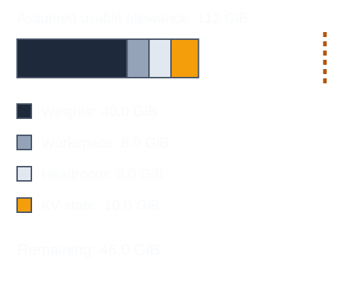
Illustrative baseline: 40 GiB weights, 8 GiB workspace, 8 GiB reserved headroom, and 10 GiB KV for one 32,768-token request. The assumed usable allowance is 112 GiB.
One conversation at the worked 131,072-token length needs about 40 GiB of KV payload. It fits this simplified ledger with some remaining room. Two unrelated conversations of that length need about 80 GiB of KV payload, exceeding the allowance before additional per-request overhead.
At the worked 32,768-token length, four independent requests need about 40 GiB of KV payload. That appears possible in the ledger, but it still needs runtime verification: batching may change workspace use, and the serving engine may reserve context differently from this dynamic estimate.
This is the answer to “it loaded, so why did it fail later?” Loading proves that one allocation stage succeeded. It does not prove that all permitted conversations can reach their maximum lengths simultaneously.
Concurrent requests do not usually duplicate every weight
A server batching requests against the same resident model can commonly share its weights. Each unrelated sequence still needs its own attention state. Starting a separate process per colleague may duplicate the weights as well, making process architecture part of the capacity decision.
Prefix sharing can reduce duplicate state when requests have an identical reusable beginning and the engine supports shared blocks. Suppose the invoice instructions and repository snapshot form a shared beginning, after which two people ask different questions. Their shared blocks may occupy memory once, while each suffix grows separately.
That is an optimization to verify, not capacity to assume. Different model settings, a changed repository snapshot, different routing, or an evicted prefix can remove the sharing opportunity. Plan the service’s admission policy so a cache miss does not suddenly make an accepted workload impossible.
There is also a difference between concurrent users and concurrent generations. Several people can use a queued service with only one active generation. That saves active memory at the cost of waiting. A capacity plan should state both the active-request limit and the expected queue behavior.
Weight quantization and KV quantization are separate knobs
Changing the weights to a smaller format does not automatically change the cache format. You can have low-bit weights with a higher-precision KV cache. This surprises people because the model filename usually advertises weight quantization prominently, while cache configuration lives elsewhere.
In the worked example, reducing cache elements from two bytes to one would halve the raw payload: the 40 GiB case becomes 20 GiB before scales and layout overhead. That is another illustrative calculation, not a promise that every backend supports a suitable one-byte cache or preserves task quality with it.
Quantized cache support may vary by key versus value storage, attention implementation, and model architecture. Verify the exact engine flags and test the invoice question at the intended context depth. A setting that loads successfully but corrupts long-context behavior is not a successful capacity improvement.
Offloading state to CPU memory or another tier can also save accelerator allocation. The price is data movement and possibly extra synchronization. On a shared-memory system, the relevant question is the actual allocation and access path, not simply whether a setting contains the word “CPU.”
Dense and mixture-of-experts models answer different size questions
A dense transformer generally uses its dense parameter arrays for each token. A mixture-of-experts model, or MoE, routes tokens through selected expert subnetworks. Fewer active parameters can reduce work per token compared with activating every expert.
But “active parameters” are not a weight-storage budget. If different tokens can choose different experts, those expert weights must remain available somewhere. An offloading system may move them between tiers, which creates another performance question. Total stored parameters, active parameters, and resident bytes are three different quantities.
Nor can you infer KV size from the expert count alone. Use the actual attention architecture. A large MoE and a smaller dense model can have very different relationships between weight memory, attention memory, and generation speed.
For our invoice assistant, choose a candidate because its answers and supported runtime suit the work. Then measure its allocations. Marketing shorthand such as “small active size” cannot replace that order of operations.
Optional experiment: make the budget visible
On a disposable local server, measure memory after model load and then at increasing retained context lengths. Keep output length fixed. Add a second independent request, then test a pair with a shared beginning if the engine supports prefix sharing.
Record input and output tokens, allocated and peak memory, time to first token, output speed, cache hits, total completion time, and whether the request queued, failed, or triggered offload. Keep a separate correctness check for the invoice policy. Label observations our measurement, with the exact runtime and settings.
Stop before destabilizing the workstation; use the server’s documented context and concurrency limits. The goal is to find a safe operating envelope, not force the operating system into an out-of-memory event.
If the weights fit but your intended conversations do not, you now have concrete choices: reduce irrelevant context, reduce active concurrency, test supported cache quantization, or add capacity. Next we examine what happens when that extra capacity sits behind a cable. For the wider local-versus-hosted choice, return to Choosing Your AI Stack.

Running AI Yourself: Where the Time and Memory Go
6 parts in this series.
Six practical explainers following a coding assistant from its first repository question to a shared local service: inference, memory budgets, PCIe topology, prompt caching, scheduling, and hardware placement.
- 01What Actually Happens When You Send an AI Prompt?previous
- 02Your Model Fits. Why Does Your Conversation Run Out of Memory?← you are here
- 03Two GPUs, One Narrow Cable: Where Does the Traffic Go?up next
- 04Stop Reprocessing the Same Prompt: Caching for Coding Agents
- 05Prefix Caching, Chunked Prefill, and the Trouble with Chunks
- 06One Halo, Several Halos, or a Desktop Full of GPUs?
What did you take away?
Thoughts, pushback, or a story of your own? Drop a reply below — I read every one.
Comments are powered by Disqus. By posting you agree to theirterms.